- ACS 5-year estimates
-
The American Community Survey's five-year rolling samples, the successor to the
Decennial long form after 2000. Each release pools sixty months of interviews, so
"ACS 2020-2024" describes the whole window rather than a moment, and consecutive
windows overlap. Two consequences run through this work: comparing an early window
with a late one understates change wherever the windows share years, and every
estimate carries a published Margin of error which becomes the cell's
Instrument precision.
- Acceptance gate
-
The test a candidate Fill table value must pass before it is allowed into the Chart. A
proposed source for an Item is accepted only if, at a time point where both the existing series
and the candidate exist, they agree across counties in rank and in level: the rank correlation must
clear a threshold calibrated to the item's own decade-to-decade persistence, and the ratio of
medians must sit near one. The self-calibration matters, because demanding that a filled series
track the panel more tightly than the panel tracks itself would reject good data.
A gate that a defective series can bypass is worth naming, and one did: see
Part-year base defect. The stricter form, used when the derivation has a known right answer, is
Verify-then-emit.
- Algorithmic information theory
-
Description length measured in programs rather than in codes for distributions: the
complexity of an object is the length of the shortest program that outputs it, a quantity that
does not depend on a chosen parametric family except up to an additive constant. Founded
independently by Solomonoff, Kolmogorov and Chaitin in the mid-1960s.
It is uncomputable, so every practical use is an approximation — here a Two-part code over
one model class. But it is the criterion being approximated, and it is what the
Core methodological thesis appeals to at the System identification stage, where the object
sought is a generating law rather than a description of a sample. See Solomonoff induction
and Algorithmic statistics.
Solomonoff (1964); Kolmogorov (1965); Chaitin (1966).
- Algorithmic statistics
-
The branch of Algorithmic information theory that gives formal meaning to the split a
Two-part code performs: separating an object's meaningful information — the model, the
lawlike part — from its accidental information, the residual that is incompressible noise
relative to that model. Kolmogorov's structure function makes the trade-off precise and picks out
a minimal sufficient statistic: the smallest model leaving a residual indistinguishable from
noise.
This is the warrant for the move the whole project rests on — treating the model half of the
code as the object of interest and the residual as nothing but measurement at
Instrument precision. Without it, "the model got shorter" is a statement about an arbitrary
partition. Kolmogorov (1974); Gács, Tromp and Vitányi (2001), "Algorithmic
Statistics".
- Autonomy
-
The property that makes a relation usable for policy: it continues to hold when
something acts on the system rather than dissolving into the correlations that
produced it. Named by Frisch in 1938 and developed by Haavelmo in 1944, it predates
Pearl's do(C) by about half a century, and Pearl credits Haavelmo for it. It is
the Warrant this project appeals to: the claim is not that a graph was drawn
correctly but that a measured Recurrence held fixed across decades and across US states. Frisch (1938), memorandum on autonomy; Haavelmo (1944),
"The Probability Approach in Econometrics".
- Backfill
-
Supplying values for time points where an Item exists as a concept but not as a
published number, by locating the same construct in another source and passing it
through the Acceptance gate. Distinct from imputation: a backfilled cell is a
measurement from elsewhere, not a model output. The Pullback does imputation
proper, and the two are kept separate so that a claim about code length is never
resting on the model's own fabrications.
- Becker specialization model
-
Gary Becker's account of marriage and fertility as household production: gains from
marriage arise from specialization, and children are time-intensive goods whose cost
rises with the wage of whoever supplies the time. It predicts that rising women's
wages lower fertility through the Opportunity cost of children and weaken the
specialization gain from marriage. It is the standard economic frame for the question
this project asks, and the frame the Contrast on women's participation is designed
to probe. Becker (1973), "A Theory of Marriage"; (1981), "A
Treatise on the Family".
- Blocked code length
-
Accumulating a code length one block of rows at a time under gradient checkpointing,
so that the (rows by items by mixture components) intermediates are never all resident
at once. A code length is a sum over cells, so blocking is identical arithmetic; what
changes is that each block is recomputed during the backward pass instead of being
held. Introduced when the widened panel exceeded the GPU by about a hundred megabytes.
Verified identical at fixed parameters: gradient cosine similarity $1.000000000000$,
relative difference $3.7\times10^{-7}$. Runs still diverge over many optimizer steps,
because floating-point summation order differs and gradient descent amplifies it.
- Canonical variate analysis
-
A subspace identification method that chooses latent coordinates to maximize
correlation between the past and the future of a series, rather than to maximize
explained variance. The distinction matters here: a variance-ranked decomposition
keeps whatever is large, while a predictive-state decomposition keeps whatever carries
information forward, and those are not the same coordinates. See Latent state.
- cause(C)
-
The intervention operator used throughout this work, deliberately not written
do(C). $\mathrm{cause}(C)$ is the Minimum-norm displacement of a county's
Latent state that realizes condition $C$ in the decoded observables, with every
other observable co-moving as the manifold requires, propagated forward by the
identified Recurrence and decoded with intervals.
Nothing is severed and there is no graph. Because the Cross-section as system state
is the whole county record, a condition on one Item necessarily moves others, and
those Co-moves are reported rather than assumed away. Minimum norm is a stated
choice, not something the data forces. The Warrant for reading the result as
causal is measured Autonomy, not graph surgery.
- Cell
-
One number in the Chart, at the intersection of a row and a column — the spreadsheet sense
of the word. A row is one county at one time point; a column is one Item, a property of
counties. The cell where they meet is that county's value of that property in that year: Webb
County, median home value, 2020. It is the Panel's atom --- what plain usage would call a
datum --- and the unit everything in this project is counted in.
The Panel version reported here is 25,168 rows (3,146 counties at eight time points) by 777
columns: 19,555,536 cells, of which 9,280,572 are observed and the remaining
10,274,964 were never measured. That is 47.5% — the table is about half empty, and the half that
is empty is not missing at random, since a column exists only for the years its source published
it.
Three consequences run through the method. Each cell carries its own Instrument
precision, the published Margin of error of that county's estimate of that item in that
year, so the residual code is summed cell by cell at cell-specific precision rather than at one
tolerance for the table. Unobserved cells contribute nothing to the code, and are not filled in
first and coded afterwards; Observed-cell MDL is where that distinction is argued, and it
decides whether a code length means anything at all on a table this empty. And every code length is reported per cell, because a total in bits is
uninterpretable across tables of different size while bits per cell can be compared with the
Per-item null and the Oracle.
- Chart
-
The assembled numerical object the model trains on: a matrix of county-time rows by
Item columns, with a parallel matrix of per-cell Instrument precision values
and a boolean mask of which cells are observed. Built by one function whose flags
record every curation decision, so that a model checkpoint plus its configuration
reproduces the exact chart it saw. Values are stored under the log1p / s95
transform. Distinguished from the County-decade panel, which is the underlying
design; the chart is that design rendered into arrays.
- CIPSEA
-
The Confidential Information Protection and Statistical Efficiency Act, re-enacted as Title III
of the Evidence Act. It protects records collected for statistical purposes from disclosure or
use against the respondent, and establishes a presumption that such data be made accessible to
qualified researchers for evidence building. Both halves matter here: the protection is why a
corpus cannot simply be released, and the accessibility presumption is why a
Sealed-corpus benchmark is administratively reachable without new legislation.
- Closed system
-
A model in which every quantity that moves the system state is itself part of the system state, so nothing is
supplied from outside. This project is not closed, and the consequence was measured: the
shared displacement is either a free parameter per period or a linear function of national series
imported from elsewhere, and it is the only component of the fitted system that fails to
extrapolate. Having refused the Exogenous variable at county level, we reinstated it at the
aggregate.
The remedy is concrete. Eight of the twelve national series used are aggregates of the county
cross-section and should be computed from the system state; the remaining four -- consumer prices, real
output per capita, the long mortgage rate, federal debt to output -- are genuinely outside a
county panel and should be promoted to state variables carrying their own dynamics rather than
imported. A closed system has no shared displacement to extrapolate, because the aggregate is
generated rather than assumed.
- Cohort and period fertility
-
Period fertility describes what happened in a calendar year across all ages; cohort
fertility describes what a group born in the same year eventually did. The
Total fertility rate is a period measure, and it can fall and recover purely
because births are postponed, with completed cohort fertility barely moving. Any claim
that a policy or a price "reduced fertility" has to say which one it means. See
Tempo and quantum.
- Co-move
-
The change an intervention induces in observables other than the one it names, because the system state is a point on a manifold and cannot be moved in one coordinate
alone. Reported alongside every cause(C) result in within-standard-deviation
units, largest first. They are the honest content of "no exogenous variables": in a
finite system the co-moves are not contamination to be purged, they are what
intervening actually consists of.
- Consistency-closed model
-
A state-space model in which the Recurrence's output must code not only the next
period's observations but also the encoder's own embedding of that next period.
Without the closure a Recurrence can score well one step ahead while its image drifts off the
manifold, so multi-step propagation becomes meaningless — which is exactly what
happened in the unconstrained joint model here, and why its multi-step effects were
withdrawn. The closure term is a Gaussian code on the latent discrepancy at its own
fitted per-coordinate scale.
- Contrast
-
An intervention stated as two conditions at once — typically move one Item and hold another
at its factual value — rather than as a single-item change. Two reasons. Substantively, a
single-item move on this manifold drags the whole labour market with it. Technically, a contrast is a difference between two system states propagated by the same Recurrence, so the shared displacement's
explicit term cancels from the difference equation — including the
Synchronization component, which is the part that does not extrapolate.
The cancellation is narrower than it looks. The base trajectory still depends
on every shared displacement applied before it, and for a quadratic map the remaining bracket
depends on that trajectory, so the shared path reaches the answer twice: through the latent
difference and through the decoder, whose percentage baseline it moves. Both routes are measured
rather than argued. Doubling the shared path at every step for thirty years moves the latent
difference by $2.8\%$. Varying only the shared path across eight scenarios
(shared_path_audit.py) moves magnitudes by a median of $0.32$ times the fitted-path
effect and holds $79$ of $84$ signs, where two scenarios leave the region the data occupy and are
dropped unread. Four of the five sign changes are median home value, a nominal-dollar item that
cannot be separated from a shared path which is mostly the price level; it is also the outcome
that changes sign between a 1980 and a 1990 base. Contrasts are conditional on a base year and a
shared path in magnitude; the family-structure directions survive both tests. See Closed
system, which removes both routes by construction.
- Core methodological thesis
-
The claim that organizes the project, and the reason code length is applied at two stages with
different standing.
Compressing a static cross-section is statistical model selection. What it exploits is
correlation among Items across counties, and no quantity of it distinguishes a cause from a
co-varying bystander. Compressing a record over time by an autonomous Recurrence is a
different act: what is shortened is the description of the process, and the thing that shortens it
is a generating law rather than a distribution over samples. The thesis is that the second is
identification of mechanism where the first is only description of correlation.
Two things have to be kept straight, and the distinction is easy to lose. First, the induction
principle at the second stage is Algorithmic information theory — shortest generating program —
not Rissanen's statistical Minimum description length, which is its computable approximation
within a fixed Family of models and is the right tool only at the Manifold autoencoder stage. Second,
algorithmic induction by itself delivers convergence of prediction, not of attribution: it
will converge using a law that is not autonomous. The causal reading requires the further
demand that the law hold in regimes it was not fitted on, which is Autonomy, tested as
Invariant causal prediction and scored by Skill. Compression supplies the candidate;
invariance out of regime is what promotes it to a mechanism.
- Corpus selection
-
Deciding which instruments enter the record at all. No criterion defined over a fixed corpus can
make this decision, because the alternatives differ in what they contain rather than in how well
they are described -- which is why it survives every refinement of the criterion and is the
irreducible residue of the Core methodological thesis. Compression scores descriptions of a
record; it is silent on the design of the study that produces the record.
The Instrument-proximate corpus rule does not solve it but sharpens it, converting ``which
processed products do we trust'' into ``which instruments do we read'', which is a question about
the world rather than about somebody else's judgment calls.
- Panel version
-
One of the successive assemblies of the County-decade panel, each admitting data the last
one lacked: 525 items, then 770 once the Reference-year column defect was repaired, then 777
with the 2011-2015 window added. Comparing results across versions is how this project measures
whether a finding is a property of the world or of what happened to be in the file — the primary
Contrast keeps its sign across all three, while its magnitudes attenuate monotonically.
Never called a ``generation''. This project studies intergenerational
causation and reports an outcome named the next generation's bachelor's share, so that word is
reserved for people. The collision is the same hazard as System state against US state and
Family of models against Family household: system identification and demography grew their
vocabularies separately, and applying one to the other keeps producing it.
- County-decade panel
-
The design underlying the Chart: roughly 3,140 counties observed at seven time
points from 1970 to 2024, each carrying several hundred Items. Decadal spacing was
a deliberate choice — the time constants of fertility and family formation are
measured in decades, and coarser spacing sharply reduces missingness — later extended
with two sub-decade points from the ACS 5-year estimates to reach 2024. Counties
are keyed by STCOU.
- Coverage
-
The fraction of observed cells whose true value falls inside the model's nominal
ninety-percent predictive interval. A calibration check rather than an accuracy one: a
model can have short code length and still lie about its own uncertainty. Values near
0.92 to 0.93 here, slightly conservative.
- Criterion of merit
-
A rule for saying which of two models of the same record is better, computable without discretion. Model
selection is the primary act and data selection follows from it: a source or a cleaning step
earns its place when the account it makes possible costs fewer bits than the account without it,
which is a question the criterion answers and no amount of deliberation about
corpus selection can. The
Evidence Act created access and governance for federal evidence building and defined no such
rule, so the question falls to expert judgment exercised inside privileged access. This project
proposes total description length at Instrument precision as the missing criterion: a number
in bits, with no tuning constant, no protocol to negotiate and no test set to select.
- Cross-section as system state
-
The modeling stance that a county's system state at a time is its entire observed
cross-section — every Item at once — rather than a handful of variables chosen in
advance. The alternative, selecting a few "drivers" and calling the rest noise, imports
a causal hypothesis before any measurement occurs. Stated in this project as the
refusal of the Exogenous variable: in a finite universe nothing is outside the
system, so the burden is on any proposal to *remove* a coordinate, not to include one.
The cost is dimensionality, paid for by the Manifold autoencoder.
- Decennial long form
-
The sample questionnaire sent to roughly one household in six at each decennial
census through 2000, and the source of everything the short form did not ask: income,
education, labor force, housing value, detailed marital status. Discontinued after
2000 and replaced by the ACS 5-year estimates, which is why so many series in this
panel change source at the 2000-to-2010 step and why that single splice receives
disproportionate scrutiny.
- Denoising mask
-
Randomly hiding a fraction of the observed inputs during training while still
requiring the model to code them. It prevents the encoder from copying inputs to
outputs and forces the Latent state to carry information that generalizes across
coordinates, which is also what makes the Pullback usable as imputation.
- Design factor
-
The ratio by which a survey's true standard error exceeds the simple-random-sampling
(binomial) value, because of clustering, stratification and weighting. Rather than
assume one, this project measures it: the same shares exist in the panel at points
where the ACS 5-year estimates publish a Margin of error, so the ratio of that
sigma to the binomial sigma on the same counties gives the factor, measured at 1.59 and
applied to every year of the NHGIS-derived series.
- Developmental map
-
The component of the Recurrence that acts on county-specific motion, after the
Synchronization displacement shared by all counties is removed — a part of the transition law,
never the whole of it. Fitted in quadratic form it is measurably invariant across decade regimes;
fitted linearly it is not, curvature being read as time-variation when the form is forced to be
linear. That
invariance is the measured Warrant for the causal reading. The name follows the
developmental-trajectory literature in single-cell biology, where the same problem
arises: recovering a process from a population observed without a clean time axis.
- Disclosure avoidance
-
What a statistical agency does to stop a published table from identifying an individual:
suppressing small cells, rounding, swapping records between similar areas, and more recently
injecting calibrated noise under Formal privacy. It is not a marginal nuisance for a county
panel — it sets a hard ceiling on what county tabulation can ever show, and it binds hardest in
small counties, which is exactly where this panel is already thinnest.
It now also sets the panel's end date. As of the Census Bureau's August 2026 updates no release
date has been set for the 2021-2025 ACS 5-year estimates: the Bureau is working out how to
publish them under a Department of Commerce order, DAO 216-26, and has said it is seeking a
compliant method for release later in 2026. Until then the County-decade panel ends at 2024.
- Displacement
-
A movement of a unit's Latent state, in the coordinates the Manifold autoencoder learned.
The word is never used bare in this project, because two displacements with opposite standing are
in play at once. The shared displacement is the period-by-period motion every unit
receives together (Synchronization); it is supplied from outside the system, it does not
extrapolate, and it is the reason level forecasts are not quoted. The minimum-norm
displacement is what cause(C) computes: the smallest move of one unit's system state that realizes a
stated condition (Minimum-norm displacement).
A Contrast is built to cancel the first and report the second, which it does for the
explicit term but not for the trajectory behind it — measured, magnitudes move by a median of
0.32 times the fitted-path effect while 79 of 84 signs hold. See Contrast.
- do(C)
-
Pearl's intervention operator: setting a variable to a value by deleting the edges
into it in a causal graph, so the intervened variable no longer responds to its former
parents. Its warrant is the correctness of the graph. This project uses cause(C)
instead, not as an objection to Pearl but because the invariant structure here is a
Recurrence rather than a DAG, and there is nothing to sever. Both formalize
Autonomy; the difference is what kind of object is assumed autonomous. One
practical asymmetry: a recurrence's autonomy is testable out of sample, and is tested
here. Pearl (1995, 2009).
- Easterlin hypothesis
-
Richard Easterlin's argument that fertility responds to young adults' income
relative to the material expectations formed in their parents' households,
not to absolute income. Large cohorts crowd the labor and housing markets, depress
their own relative position, and postpone or forgo children; small cohorts do the
reverse. It is the closest thing in the existing literature to
Outbidding the economy, and it is a relative-price argument, which is why the
Contrast rather than the level forecast is the right instrument for it.
Easterlin (1980), "Birth and Fortune".
- Ecological fallacy
-
Inferring about individuals from relationships measured on groups. A county where
women's education and childlessness both rise tells you nothing directly about whether
the educated women are the childless ones. This is the standing caveat on everything
here: the analysis is of counties as units, and every effect is an effect on a county,
not on a person. Stating it does not dispose of it.
Robinson (1950), "Ecological Correlations and the Behavior of
Individuals".
- EDURAT
-
The ratio of women's to men's share of bachelor's degree or higher among adults 25
and over, with EDUFBA and EDUMBA the two component shares. A ratio rather than a
difference, for three reasons: it is dimensionless and so comparable across counties
at very different attainment levels, it stays positive and survives the
log1p / s95 transform, and a ratio is a difference of logs, which is the geometry
the Chart already works in. At the median county it runs 0.749 in 1970 to 1.196 in
2024, crossing one between 2000 and 2010. Relevant to Educational hypergamy.
- Educational hypergamy
-
Marrying up the educational ladder; hypogamy is marrying down, homogamy marrying
level. The historical pattern of women marrying men with more education has inverted
in most rich countries as women's attainment overtook men's, and a literature asks
whether the adjustment in preferences has kept pace with the arithmetic. When
EDURAT exceeds one, a strictly hypergamous norm becomes arithmetically
unsatisfiable for some fraction of women — a structural Marriage squeeze in
education rather than in numbers.
- Effective sample size
-
The number of independent observations a correlated sample is worth. Counties are
spatially correlated and a county's successive decades are strongly autocorrelated, so
15,730 transitions are not 15,730 independent facts. Every invariance verdict here is
scored against an effective count rather than a raw one, which is what keeps
"the Developmental map varies across decades" from being a statement about sample size.
- E-folding time
-
The time for a mode of a linearized Recurrence to decay by a factor of $e$, computed
from the eigenvalue modulus. Reported here per latent direction to give the persistence of the
identified dynamics in years: the slowest directions have e-folding times of centuries,
which is a way of saying the county system has very long memory and that a thirty-year
horizon is short relative to its own relaxation.
- Evidence Act
-
The Foundations for Evidence-Based Policymaking Act of 2018 (P.L. 115-435). Title I directs
agencies to build evidence and appoint evaluation and data officers; Title II, the OPEN Government
Data Act, establishes a presumption that public data be open and machine readable; Title III
re-enacts CIPSEA and creates a presumption of accessibility for statistical purposes. The
committee it established recommended the National Secure Data Service.
What it does not contain is a Criterion of merit. It is machinery for getting data to
analysts, and it is silent on what distinguishes better evidence from worse -- so that judgment
falls to peer review and agency expertise, neither contestable from outside the access regime.
See Privileged-access replication.
- Exogenous variable
-
A variable treated as determined outside the system under study, so that it can be
varied without the model having to explain it. The organizing objection of this
project is that in a closed finite system there are no such variables, and that
designating some is a prior about causal structure wearing the costume of a modeling
convenience. The alternative adopted here is the Cross-section as system state. The
price is that nothing can be "held constant" for free: holding something fixed is
itself an intervention, which is why interventions are posed as a Contrast.
- Family household
-
A census unit: a householder living with one or more people related by birth, marriage or
adoption. Family structure supplies several of this project's outcomes — married couples with own
children under 18, female-headed families with own children, and the derived FAMMCH and
FAMFCH shares — and family formation is the substantive process the whole study is about.
Not a Family of models. The two senses collide in this work: the most robust
substantive finding concerns families of the first kind, and the frankest methodological limitation concerns a family of models. Bare ``family'' is therefore never used.
- Fill table
-
A plain table of STCOU, item, year, value, delta rows produced by one
curation script from one source, which the Chart builder merges in. Keeping each
source in its own fill, merged in a fixed order with the last writer winning, means a
source can be added, corrected or withdrawn without touching the others, and the
provenance of any cell is a matter of record rather than reconstruction. Items not
already in the panel become new columns.
- Formal privacy
-
A Disclosure avoidance approach that bounds, by a stated and published parameter, how much
any one record can influence a released statistic — differential privacy and its relatives — as
against traditional methods like swapping, whose protection is real but unquantified. Used for the
2020 decennial census. Whether the ACS will move to it is not yet known; that is the open question
behind the 2025 delay.
Two consequences for this work if it does. A published Margin of error would then describe
sampling error alone, so Instrument precision would understate total error unless the injected
noise variance is added to it — and because a formal mechanism publishes its parameters, that
correction is exactly computable, which swapping never permitted. And the change would be a method
change at a splice, the failure mode this panel has already been damaged by once, so any 2025 point
must clear the Acceptance gate against a 2024 point produced under the old regime rather than
being appended to it.
- Function library
-
The set of candidate functions of the Latent state from which the
Recurrence is built — here constants, linear terms and pairwise products. Fitting
a Recurrence means selecting a sparse combination from the library by code length rather than
by a significance threshold, so that adding a term must pay for itself in bits. The
approach is shared with sparse-regression system identification.
- Gaussian mixture head
-
The decoder's output layer: for each Item it emits a small mixture of Gaussians
rather than a point estimate. This is what lets the residual term be an honest code
length — the number of bits to transmit the true value given the model's distribution
at that cell's Instrument precision — and what lets asymmetric and multi-modal
item distributions be coded without transformation tricks.
- Held-out transition
-
A set of period-to-period transitions excluded from the training objective and kept
for scoring. Naming the year that a transition starts identifies it: holding
out 2010 removes the 2010-to-2020 step. This is the only honest test of the
Recurrence, because the Pullback can always code a period it has seen. Scored
against Persistence, Oracle and the Per-item null; see Skill.
- Hutter Prize
-
A standing prize for lossless compression of a fixed corpus of English Wikipedia, premised on the
claim that compression and understanding are the same problem. Two features are load-bearing for
the proposal here: the corpus is raw, markup and errors included, so that cleaning is
part of the submitted compressor rather than unscored prologue; and the score is a single number
that admits no discretion. The macrosociological analogue is a Sealed-corpus benchmark, which
adds only that the custodian runs the program because the corpus cannot be released.
- In-region fraction
-
The share of counties whose intervened system state still lies within the region of the
manifold where data exist. A cause(C) result with a low in-region fraction is
describing counties that do not exist, and is reported and flagged rather than quoted.
The clearest instance here: after per capita income was corrected to real dollars, a
one-standard-deviation income intervention fell to 2 to 7 percent in-region, because a
full cross-county standard deviation of income is simply outside the region the data occupy.
- Instrument precision
-
The resolution at which a cell's value is actually known — the published
Margin of error for a survey estimate, the rounding step for a tabulated count,
a propagated combination for a derived quantity. Carried per cell alongside the value,
and it is what makes the residual term a code length rather than a likelihood: coding
a number to infinite precision costs infinite bits, so the question "how many bits does
this model save" only has an answer once you say how precisely the data are known.
- Instrument-proximate corpus
-
The rule that a corpus should be held as close to the measurement instrument -- mechanical like a
thermometer, or institutional like a vital-statistics registry -- as law allows, so that every
cleaning step falls inside the submitted algorithm rather than upstream of it.
The argument is measured, not aesthetic. Per-capita normalization of a median costs exactly
$-0.0000$ bits when the denominator is in the corpus, because the corrupted column is then an
invertible function of the clean one: as a step inside a program the choice is free and legible,
and the criterion is rightly indifferent. Applied before the corpus the same step is
unfalsifiable, and the column silently denotes something other than its name -- which is how the
Median per-capita defect survived. Everything upstream of the boundary is axiom.
- Invariance
-
The property that licenses reading a fitted relation as something one may act on rather than
merely read off: the same relation holds, with the same coefficients, across environments that
differ in every other respect (Regime). It is the content of Autonomy in Frisch and
Haavelmo, of the Lucas critique's demand, and of Invariant causal prediction's
identification criterion.
Tested here by Minimum description length, not by a significance test: a map is invariant
across a set of regimes when fitting it separately per regime does not pay for its own extra
Parameter code. On the current model the quadratic Developmental map is invariant across
all six decade regimes and the linear map across all 41 US-state regimes. The verdict is recorded
per run and printed on every figure (Warrant), so a weakened claim travels as a weakened
claim.
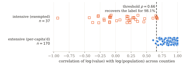
- Intensive and extensive items
-
An extensive Item scales with county size — a count of households, an aggregate
payroll — and must be divided by population before counties are comparable. An
intensive item is already a ratio, a rate, a median or an average, and must not be.
Getting this wrong in either direction produces a quantity with no meaning, and it
went wrong twice here: see Median per-capita defect. The unit code alone cannot
decide it, since dollars label both an aggregate payroll and a median income, so the
item description has to be consulted; see Prenormalized item.
- Invariant causal prediction
-
An identification strategy that takes invariance across environments as the
criterion for causality: a relation that holds unchanged across regimes is a candidate
causal relation, and one that does not is not. It supplies the formal basis for what
this project measures when it asks whether the Developmental map is the same across decades and across US states. Peters, Bühlmann and Meinshausen (2016),
"Causal inference by using invariant prediction".
- Item
-
One measured quantity in the panel, identified by a short code — HSG490
for median owner-occupied home value, VST020 for births per thousand — and
carrying a unit indicator, a description and a decimal resolution. The codes come from
USA Counties; constructed measures added here use mnemonic codes of the same shape.
Items are the columns of the Chart.
- Latent state
-
The low-dimensional coordinates the encoder assigns to a county at a time point —
thirty-two numbers standing in for several hundred Items. The claim that this is a system state rather than a summary is an empirical one, and it is tested: a system state must support a Recurrence that predicts the next period, which is what the
Consistency-closed model enforces and the Held-out transition scores.
- LFPRR
-
The ratio of women's to men's labor force participation among adults 16 and over,
with LFPRF and LFPRM the components. At the median county it runs 0.507 in 1970 to
0.868 in 2024 — women's participation rising from 36.9 to about 55 percent while men's
falls from 73.7 to 63.5. Together with EDURAT it is the measured form of the
change whose consequences this project asks about.
- Linkage
-
Joining records on the same person or household across agencies -- tax to survey to program to
education. It is what makes restricted access valuable and it is the most tightly governed
operation in federal statistics, because the governing statutes differ by agency and were not
written to compose. A Sealed-corpus benchmark needs the linked corpus to exist; creating it is
a political question the mechanism does not answer, and it is the largest real obstacle to the
proposal.
- log1p / s95 transform
-
The Chart's storage transform: $y = \log(1+x)/s_{95}$, where $s_{95}$ is the
95th percentile of the observed $\log(1+x)$ values across the whole chart. The
logarithm puts items spanning eight orders of magnitude on comparable footing and makes
ratios into differences; the single global scale keeps one common unit so that bits per
cell means the same thing everywhere. Instrument precision is propagated through
it as $\delta y = \delta x / ((1+x)\,s_{95})$. It requires non-negative values, which
is why derived measures are defined as ratios rather than signed gaps.
- Lucas critique
-
Robert Lucas's 1976 argument that relationships estimated from historical data will
change when policy changes, because the behavior generating them was optimized against
the old policy. It is the dynamical statement of Autonomy: a relation that is not
autonomous breaks precisely when you act on it, which is precisely when you wanted it.
The reason this project insists on out-of-sample invariance testing rather than fit.
- Manifold autoencoder
-
The encoder-decoder pair that takes a county's full observed cross-section to a
Latent state and back. "Manifold" rather than "compression" because the object of
interest is the learned surface the counties lie on: the Recurrence is defined on
it, cause(C) moves along it, and the In-region fraction asks whether a proposed
intervention stays on it. Trained by Minimum description length, not by
reconstruction error.
- Margin of error
-
The Census Bureau's published sampling uncertainty for a survey estimate, given at
the 90 percent level, so a standard error is the margin divided by 1.645. Converted to
Instrument precision for every cell sourced from the ACS 5-year estimates.
Where no margin is published, a standard error is derived from the sample fraction and
inflated by a measured Design factor.
- Margin over null
-
Bits per cell of the model minus bits per cell of the Per-item null, a negative
number when the model helps. The comparison that survives a change in the item set:
absolute bits per cell fall simply by adding predictable items, so two models
built on different panel versions can only be compared on their margins, and even
then only cautiously, since the null itself changes character when the added items are
highly persistent.
- Marriage-market sex ratio
-
Men per woman in the age bands that actually marry each other, built from
single-year-of-age county populations with the male window offset upward by the
observed marriage-age gap rather than by a fixed constant, so that the measure tracks
the gap as it changes. MSR0 is the unoffset version for comparison. The quantitative
form of the Marriage squeeze; the age offset is taken from
Singulate mean age at marriage.
- Marriage squeeze
-
An imbalance in the number of available partners at marriageable ages, arising
mechanically when cohort sizes change and men marry younger women. Guttentag and
Secord's extension argues that the scarcer sex gains dyadic power while the more
abundant sex faces worse terms, with consequences for marriage rates, family-household stability and fertility. Measured here as the Marriage-market sex ratio; the education
analogue is under Educational hypergamy.
Guttentag and Secord (1983), "Too Many Women? The Sex Ratio
Question".
- Median per-capita defect
-
A curation bug in this work, named because it recurred. Per-capita normalization was
keyed on the unit code alone, and dollars are a count unit, so four dollar-median
housing items were divided by county population — producing median-value-per-resident,
a quantity with no interpretation. Found and fixed; then found again in a second form
where the guard matched "average" and "median" but not "mean" or "per capita", which
put per capita personal income, a Contrast variable in every causal result to that
point, through the same mill. Both are instances of Intensive and extensive items
being misclassified. Recorded here because the lesson is that a defect of this shape is
invisible in fit statistics and only shows up when someone reads the numbers in their
own units.
- Minimum description length
-
Rissanen's principle that the best model is the one that, together with the data encoded using
it, yields the shortest total description. It converts model selection into a measurement in bits
with no free parameter for how much complexity to tolerate: a model earns a parameter only if that
parameter buys back more bits than it costs. Implemented here as a Two-part code.
It is a statistical principle, and its scope in this project is the first stage only.
It selects within a parametric family, and it is the right tool for the Manifold autoencoder,
where the task is to compress a cross-section and the structure being exploited is correlation
among Items. It is not the criterion appealed to at the System identification
stage: there the object is a generating law, the governing principle is
Algorithmic information theory, and this is its computable approximation rather than its
equivalent. Treating Rissanen as the criterion at both stages collapses the distinction the
Core methodological thesis exists to draw. Rissanen (1978), "Modeling by
shortest data description".
- Minimum-norm displacement
-
Of all the latent moves that would realize a stated condition in the decoded
observables, the shortest one. It is the choice that makes cause(C) well defined,
since infinitely many latent states satisfy a condition on a few coordinates, and it is
a choice: it encodes an assumption that an intervention disturbs the system state as little as it can, which the data do not establish. Stated on every figure for that
reason.
- Family of models
-
The class of models a description length is minimized within — here a Manifold autoencoder
of stated width and depth with a Gaussian mixture head, plus a Recurrence built from a
Function library. The choice is not free and the criterion cannot price it: two-part
Minimum description length ranks models inside a family of models and is silent about which family of
models was chosen, which is the computable approximation's distance from Algorithmic information theory,
where description length is measured over all programs.
Measured sensitivity: across eight architectures spanning a sixteen-fold range of latent width,
total description length varies by $1.51\%$, so the reported code lengths are not an artifact of
one lucky choice. That is a statement about architecture within a family of models, not about the choice of family of models.
Not a Family household. See that entry for the convention keeping them
apart.
- National parameterization
-
Modeling the Synchronization component as a function of a few national time
series rather than as a free displacement per decade, in the hope that it would then
extrapolate to an unseen decade. It does not. Held out, the extrapolated national
displacement coded the next decade at 27.9 bits per cell against 14.0 for assuming no
shared motion at all — a linear function of national components fitted on three decades is
worse than nothing. Recorded as a negative result: level forecasting from a county's system state is unsupported here, which is why the project reports a Contrast instead.
- National Secure Data Service
-
The secure enclave for evidence building recommended by the advisory committee the
Evidence Act created: a facility where approved analysts compute on restricted records that
never leave it. It is the institutional vehicle a Sealed-corpus benchmark would run inside,
which is why that proposal requires no new legislation -- the enclave, the confidentiality regime
and the mandate already exist. What is missing is a published number and an open submission
queue.
- NHGIS
-
The IPUMS National Historical Geographic Information System, which republishes US
census tabulations from 1790 onward with consistent codes and documentation, through an
API that builds extracts to order. Its Time series tables are the reason the
sex-split education and marriage-age series in this panel run from 1970 instead of
2000. Use requires registration for the NHGIS collection specifically and a citation.
Schroeder, Van Riper, Manson, Cooper, Krause, Kugler, Zhu and
Ruggles, IPUMS NHGIS Version 21.0, doi 10.18128/D050.V21.0.
- Nominal integration
-
Linking geographic units across time by their names and codes, disregarding boundary
changes — as opposed to geographically standardized integration, which interpolates
every year onto one census's boundaries. Nominal is the right choice for a
STCOU-keyed county panel, since counties rarely change shape and interpolation
would introduce error everywhere to fix a handful of cases. Its failure mode is a code
that means different areas at different times, or stops existing: see
Planning region gap.
- Null initialization
-
Setting the initial weights so the untrained model's output is exactly the
Per-item null — each item a Gaussian at its own mean and variance. Epoch zero then
scores the null exactly, and every bit the model subsequently claims is a bit it
earned, measured from a baseline the model itself reproduces rather than from a
separately computed reference.
- Observed-cell MDL
-
Restricting the residual code to cells that were actually measured, with unobserved
inputs entering the encoder as the feature mean and contributing nothing to the loss.
The alternative — imputing, then coding the imputations — would let the model earn bits
for predicting its own guesses. With a panel about half observed, this distinction is
the difference between a code length that means something and one that does not.
- Opportunity cost of children
-
The earnings and career progression forgone by whoever supplies the time children
require. It rises with the wage of that person, which is why the standard economic
prediction is that improving women's labor market position lowers fertility, and why
the effect should be strongest for the highest-earning women. The demand side of the
same relation that Outbidding the economy describes from the other direction. See
Becker specialization model.
- Oracle
-
The code length achieved when the target period is coded from the encoder's own
embedding of that period — the model given the answer. It is the attainable
floor: no Recurrence can beat it, because it represents what the decoder can do with perfect knowledge of the system state. The denominator in Skill, and the quantity
that keeps a hard prediction problem from being mistaken for a bad model.
- Outbidding the economy
-
The question this work was built to ask, in the form the user posed it: whether
young men can outbid the economy for the fertile years of the most economically
valuable women, and what follows for the next generation. It frames family formation
as a bidding contest for a specific scarce resource — the limited fertile window of
women whose labor is most highly valued — in which the competing bidder is paid
employment. It is not standard terminology. The nearest established relatives are the
Opportunity cost of children, the Easterlin hypothesis (relative income of
young adults), and the Two-Income Trap (the bid getting capitalized into housing).
Its empirical shadow in this panel is the pairing of LFPRR and EDURAT against
family-structure and fertility outcomes, posed as a Contrast.
- Parameter code
-
The second half of the Two-part code: the bits needed to transmit the model
itself. Computed two ways here — an entropy code over quantized weight levels, used
for honest accounting, and a differentiable Laplace code at the same quantization step,
used inside the gradient so the optimizer actually feels the cost of its parameters.
Without this term nothing stops a model from spending unlimited complexity to shave the
residual. See Quantization-aware training.
- Part-year base defect
-
A second named curation bug. Every Census Population estimates vintage begins at
an April census base, so the "year" at the start of a vintage covers roughly three
months, not twelve. Births filled at the 2010 point from such a base read 3.19 per
thousand against a true 12.75 — a quarter of the real value — and it passed the
Acceptance gate because rank correlation across counties was unaffected. The
general lesson: a gate testing rank and level ratio catches a wrong shape but
not a uniform scale error in a period definition.
- Per-item null
-
The reference model in which every Item is an independent Gaussian at its own
mean and variance, with no county and no time structure. It is what the model must
beat to have learned anything at all, it is where Null initialization starts, and
its code length is the denominator of the Margin over null. A weak baseline by
design: beating it is necessary, not impressive.
- Persistence
-
The baseline that predicts no change: decode the base period's Latent state and
use it to code the target period. The one a Recurrence must beat to be worth
anything, since most of what a county is next decade is what it was last decade. It
must be computed on the same transitions being scored — mixing a persistence figure
from the training transitions with a model figure from the
Held-out transition produced a badly inflated Skill here before it was
caught.
- Planning region gap
-
Connecticut replaced its eight counties with nine councils-of-government planning regions for
federal statistical purposes, effective with ACS 2022. Under Nominal integration the old county
codes simply stop appearing, so the eight Connecticut counties had almost no observed cells at the
2024 point — and they include Fairfield and Hartford, high-income commuter counties central to the
question. Nothing was corrupted: the new region codes fail the STCOU join and are dropped, so
the cells were missing rather than wrong.
Closed. Both geographies are exact unions of the same 169 towns and a town's
five-digit subdivision code survives the redefinition, so the old counties rebuild by summing
county-subdivision tables. Connecticut's observed density at 2024 went from 0.004 to 0.290 against
0.319 nationally, 222 items across the eight counties. Nine items stay missing and should: a
published median cannot be aggregated from town medians. See Verify-then-emit.
- Population estimates
-
The Census Bureau's annual county population estimates, the source here for births,
deaths and net domestic and international migration. Published in vintages,
each revising the whole intercensal series from a fresh census base, so figures for the
same year differ between vintages and the base year is a part-period. Both properties
caused trouble; see Part-year base defect.
- Post-2020 regime shift
-
What looked like a break in county dynamics after 2020, and mostly was not. The median county
did flip from losing domestic migrants to gaining them (−1.43 to +2.38 per 1,000 per year), and
that part is real.
The headline acceleration was a sampling artifact. The original 1.66x compared a
three-year window against decade-scale motion — different sampling rates. Once the panel gained
sub-decade points, the noise-corrected county-specific rate per decade reads 0.106 (2010-2015),
0.093 (2015-2020) and 0.115 (2020-2024): post-2020 is about 1.15x the 2010s
five-year rate. Skill likewise appeared to halve only while the comparison was a decade holdout
against a four-year one; at matched sub-decade steps it is 0.59, 0.67 and 0.63. The identified law
does not measurably degrade after 2020. The entry is kept because the wrong version was quoted for
several days and stands in earlier commits.
- Prenormalized item
-
An Item whose published value is already a ratio, rate, median, mean or
per-capita figure, and which must therefore be exempt from per-capita normalization.
Detected from the item description, since the unit code cannot distinguish an aggregate
payroll from a median income. The detection pattern is a piece of curation logic worth
naming because getting it wrong is silent: see Median per-capita defect and
Intensive and extensive items.
- Privileged-access replication
-
The condition in which a finding can be checked only by someone holding the same restricted-data
clearance as its author, so that it rests on the author's standing rather than on anything a
challenger can attack. The customary remedy -- release the data -- is exactly what CIPSEA
forbids for the records that matter most.
It is a verifiability problem wearing privacy's clothes, and it does not require releasing
anything to fix. Under a Sealed-corpus benchmark an outsider who believes an official model is
wrong can beat its number without ever seeing a record. The present regime gives that outsider no
move at all.
- Pseudotime
-
An ordering of observations along a developmental trajectory recovered from the data
alone, without using the time stamps — borrowed from single-cell biology, where cells
are destroyed by measurement and no cell is observed twice. Applied here as a check,
and the check was informative in the negative: the recovered ordering correlates
strongly with calendar decade and barely at all with county-specific motion, meaning it
is picking up Synchronization, not development. Counties, unlike cells, are
synchronized by shared national conditions, which is precisely the difference that
makes the biological method not transfer.
- Pullback
-
Encoding a county's cross-section to the Latent state and decoding it back to
the original observables at their own Instrument precision, then measuring the
residual code. "Pullback" because the manifold's structure is pulled back onto the raw
data, in their own units, rather than being assessed in some transformed space where
the error metric is arbitrary.
Two things fall out. The residual bits are a direct measurement of how much
structure the manifold has captured, comparable across models. And the decoded values
at unobserved cells are a principled imputation — one that respects the joint
distribution of all items and reports its own uncertainty — which is a stronger object
than the usual conditional-mean fill.
- Quantization-aware training
-
Rounding weights to a per-group step in the forward pass while passing gradients
through to the unrounded masters — the straight-through estimator. Necessary because
the Parameter code counts bits of quantized weights: a model must be
scored at the precision at which it would actually be transmitted, and the step size
itself is re-chosen periodically to minimize total bits. Without this, the
Two-part code would be charging for a model different from the one being used.
- Regime
-
One of the environments across which Invariance is tested — a decade, or a US state. A
reserved word: it never means a policy, an administration, or a data-access arrangement, which
are the senses ordinary usage would supply. The reservation matters because the whole causal
warrant of this project is a statement about regimes in the first sense, and the Evidence
Act discussion on the same page is about arrangements in the second.
A regime is useful in proportion to how unlike the others it is: invariance across two similar
decades says little, invariance across forty-one US states and six decades says a great deal.
See Warrant and Post-2020 regime shift, whose name is a legacy of the reading it
corrected.
- Recurrence
-
The rule taking a county's Latent state at one period to the next. Here it is
the sum of a Synchronization displacement shared across counties and a
Developmental map acting on county-specific position, built from a
Function library and fitted by code length — at this stage an approximation to program length
in the sense of Algorithmic information theory, not statistical model selection; see
Core methodological thesis. It is the object whose invariance is
tested, the object cause(C) propagates along, and the object the whole project
means by "the identified system".
Naming: the recurrence is the whole transition law, the Developmental map only its
county-specific component, and "linear" or "quadratic" names a functional form fitted to either.
Bare "map" is avoided throughout, because this project's own logs and commit messages have used it
for all three.
- Reference-year column
-
A column in USA Counties labeled by the year its quantity refers to
rather than the year of the census reporting it: median household income collected in
the 1980 census is income in 1979, coded 1979. A grid admitting only exact decade years
silently dropped 245 such items from this panel — the entire income and poverty domain,
plus parts of housing, labor force and age — leaving a panel with house prices and
employment but no income levels at all. Admitting columns within one year of a decade
point recovered them, taking the panel from 525 to 770 items. One year, not two: two
would pull the 1998 and 2002 economic censuses into the 2000 point.
- SAIPE
-
The Census Bureau's Small Area Income and Poverty Estimates, model-based annual
county figures for median household income and poverty that borrow strength from
administrative records. Present in USA Counties as a separate item group. Being
model output rather than direct measurement, it is a different kind of object from a
survey estimate, and its uncertainty is not a sampling Margin of error.
- Sealed-corpus benchmark
-
The proposed mechanism: contestants submit programs rather than findings, a custodian runs
them inside the enclave, and only the resulting bit count is published. The data never move, so
confidentiality is preserved exactly; the program is public, so the cleaning algorithm is scored
rather than presumed; and replication becomes the act of submitting a rival program and beating
the number.
Four properties follow: no discretion in scoring, adversarial verification without access,
curation inside the scored object (see Instrument-proximate corpus), and symmetry -- it
exposes an analyst whose model is beaten and protects one whose model is not. Three obstacles
remain: Linkage, Corpus selection, and agency processing that is undocumented, where
Formal privacy is a gain rather than a loss because it publishes its noise parameters.
- Second demographic transition
-
Van de Kaa and Lesthaeghe's account of the post-1960s shift in rich countries:
sub-replacement fertility, later marriage, cohabitation, births outside marriage, and
a value shift toward self-realization. It supplies the descriptive backdrop for this
panel's 1970-to-2024 window and an alternative reading of the same facts — values
rather than prices. The two are hard to separate with aggregate data, which is worth
stating plainly rather than resolving by assertion.
Van de Kaa (1987); Lesthaeghe (2010).
- SEER single-year-of-age
-
The National Cancer Institute's county population files by single year of age and
sex, 1969 to the present, produced for cancer-rate denominators. Their value here is
incidental to that purpose: single-year age detail over a long unbroken span is what
makes an age-offset Marriage-market sex ratio computable at all, and back to 1969
rather than 2000.
- Shuffle test
-
Scoring the model after permuting the correspondence between rows and their latent
codes. The result should be far worse than the Per-item null, and is — about 14.4
bits per cell against a null near 9.6 — confirming that the code length depends on matching the right system state to the right county rather than on a generically flexible
output distribution.
- Singulate mean age at marriage
-
Hajnal's estimator of the mean age at first marriage among those who ever marry,
computed from the proportions never married by age rather than from marriage
registrations:
$$\mathrm{SMAM} = \frac{15 + \sum_x w_x S(x) - 50\,S^*}{1 - S^*},$$
with $S(x)$ the proportion never married in age band $x$, $w_x$ the person-years the
band contributes between exact ages 15 and 50, and $S^*$ the never-marrying share taken
at ages 45 to 54. Used here because median age at first marriage is not published per
county, while the never-married-by-age tabulations are. At the median county it runs
22.5 to 29.3 years for men and 20.7 to 27.7 for women, 1970 to 2024. Supplies the age
offset in the Marriage-market sex ratio. Hajnal (1953), "Age at
Marriage and Proportions Marrying".
- Skill
-
How far the model closes the gap between the Persistence baseline and the
Oracle floor on a Held-out transition:
$$\mathrm{skill} = \frac{b_{\text{persistence}} - b_{\text{model}}}
{b_{\text{persistence}} - b_{\text{oracle}}}.$$
Zero means no better than assuming no change; one means as good as knowing the answer.
Preferable to raw bits because it is bounded by what is attainable given measurement
noise. All three terms must be computed on the same transitions and the same items, or
the number is meaningless — see Persistence for how that goes wrong.
- Solomonoff induction
-
Universal inductive inference: weight every program consistent with the observations so far by
$2^{-\ell}$ in its length $\ell$, and predict with the resulting mixture. Solomonoff's convergence
theorem bounds total prediction error by the complexity of the true generator, so the procedure
learns any computable process from its own record, with no prior chosen by the analyst beyond the
choice of machine.
Two consequences here. It is a statement about sequences — about dynamics — which is
why it is the right frame for the Recurrence and not for a lone cross-section. And what it
guarantees is prediction, not mechanism: see Core methodological thesis for why Autonomy
has to be measured separately. Solomonoff (1964), "A Formal Theory of Inductive
Inference".
- Solomonoff's thesis
-
Distinguish two claims. Solomonoff induction's convergence result is a theorem and
wants no empirical evidence. What is empirical, and genuinely open, is whether bounded computable
approximations inherit its virtues on real problems -- that is Solomonoff's thesis proper.
The objection that there is ``no empirical evidence'' for it has been used to decline the very
instrument that would produce the evidence, which is circular: a Hutter Prize or
Sealed-corpus benchmark is the experiment. Nothing measured in this project bears
against the thesis; every failure reported here is attributable to a named violation of the
framework -- most sharply the one recorded under Closed system.
- System state
-
The dynamical object: a point in the state space whose motion the Recurrence describes. In
this project a unit's system state is its entire observed cross-section, compressed to the
Latent state, and the claim that it is a system state rather than a summary is empirical and tested---a system state must support a recurrence that predicts the next period.
Not to be confused with US state, the jurisdiction. The collision is
unavoidable in a paper whose units are counties nested in US states and whose method is state-space
identification, so bare ``state'' is never used: it is always system state or US
state. Watch for it in phrases like ``state variable'' and ``state regime'', which belong to
opposite senses.
- STCOU
-
The five-digit US-state-plus-county FIPS code used as the panel's unit key: US state times 1000 plus county. The join key for every Fill table, and the thing that quietly fails when a US state redefines its county geography — see Planning region gap.
- Step-size-aware transition
-
Carrying the length of each transition explicitly, so the Recurrence learns a
rate per decade rather than a displacement per step. Needed once the panel gained
points at 2020, 2023 and 2024: without it, a four-year step and a ten-year step would
be fitted as though they were the same motion, and the apparent slowdown after 2020
would be an artifact of the spacing rather than a fact about counties.
- STF and SF summary files
-
The Census Bureau's tabulated decennial outputs: Summary Tape Files in 1980 and
1990, Summary Files in 2000 and later. STF1 and STF2 are complete-count tabulations;
STF3 and STF4 come from the Decennial long form sample, STF4 carrying the detailed
cross-tabulations. Which file a construct lives in changes by decade — marital status
was a complete-count item in 1980 and 1990 but a sample item in 2000 — which is exactly
the kind of discontinuity a Time series table exists to absorb.
- Student loan non-dischargeability
-
The legal regime making student debt uniquely difficult to discharge in bankruptcy,
tightened in stages: the 1976 Education Amendments barred discharge of federal loans
for five years, extended to seven, and the 1998 Higher Education Amendments removed the
time limit for federal loans entirely; the 2005 bankruptcy act extended protection to
qualified private loans. The remaining route requires showing "undue hardship", which
most circuits assess through the Brunner test (1987), a standard rarely met. Relevant
because a debt that cannot be discharged is a fixed claim on household formation
decades before children are considered — the mechanism the Two-Income Trap argues
for, in a form its original analysis did not emphasize.
- Synchronization
-
The component of decade-to-decade latent motion shared across counties, decomposed into a
national part and a US state part, with the remainder being county-specific motion on which the
Developmental map acts. The separation matters because the two behave completely differently:
the developmental part is invariant across decades and usable, while the synchronized part does not
extrapolate at all — see National parameterization.
A Contrast removes its explicit term from the difference equation, which is why contrasts
are quotable where level forecasts are not — but not its trajectory dependence, which is measured
rather than assumed away.
Its measured size depends heavily on what is in the panel. Admitting nominal-dollar income and
housing items raised the national share from 0.49 to 0.76, almost entirely because prices inflate
together; that is a property of the price level, not a rise in real synchronization.
- System identification
-
The engineering discipline of inferring a dynamical model — system-state dimension,
transition law, noise structure — from observed input-output records, with the model
validated by prediction on data it was not fitted to. Its standards are the ones this project
adopts in place of the regression-and-significance convention: a system state must be shown to be a system state, a law must be shown to be invariant, and a fit that has not been tested out of sample is not a
result. See Canonical variate analysis, Held-out transition.
This is the project's second stage, and the criterion changes with it. What is being shortened
here is the description of a process, so the standard is program length in the sense of
Algorithmic information theory, not statistical model selection over a family of
distributions — see Core methodological thesis.
- US state
-
The jurisdiction counties nest within, and one of the two regime families across which the
recurrence's invariance is tested---the linear developmental map is invariant across all 41 US-state
regimes present in the panel. It also carries a share of the Synchronization: displacement
common to the counties of one US state but not to the country, measured at $0.05$ of squared decade
motion against $0.79$ national.
Not the System state. See that entry for the convention this project uses
to keep them apart.
- Tempo and quantum
-
Bongaarts and Feeney's decomposition of period fertility into quantum, how
many children are eventually born, and tempo, when. Postponement alone
depresses the Total fertility rate while it is under way and inflates it when it
stops, so an observed TFR decline can be pure tempo. Any account of falling fertility
owes an answer to which it is claiming. See Cohort and period fertility.
Bongaarts and Feeney (1998), "On the Quantum and Tempo of
Fertility".
- Time series table
-
An NHGIS product that reconciles one construct across multiple censuses and
survey windows onto a single category scheme, naming the residual incomparabilities in
the category labels themselves — for example "4 years of college (until 1980) or
bachelor's degree (since 1990)". Preferable to splicing raw STF and SF summary
files by hand, because a method change at a splice is a fabricated transition and
this panel had already been damaged once by one.
- Total fertility rate
-
The number of children a woman would bear if she experienced the current year's
age-specific fertility rates throughout her life. A synthetic period measure, not a
description of any real cohort, and therefore vulnerable to tempo distortion — see
Tempo and quantum and Cohort and period fertility. The quantity this project
began from, though the panel works with observed births per thousand and children under
five, which are measured per county where TFR is not.
- Two-Income Trap
-
Warren and Tyagi's argument that two-earner households did not gain slack but lost
it: the second income was bid into fixed commitments — above all housing in
school-district competition — leaving families more exposed to a single job loss than
one-earner families had been. It is the clearest published statement of the mechanism
behind Outbidding the economy, with the bid capitalized into house prices. Its
bankruptcy analysis centered on mortgage, medical and job-loss shocks; student debt
figures far less prominently there than its later prominence would suggest, which is
part of why Student loan non-dischargeability is tracked separately here.
Warren and Tyagi (2003).
- Two-part code
-
The concrete form Minimum description length takes here: total bits are the
Parameter code plus the residual code, the latter being the bits to transmit each
observed value given the model's predictive distribution at that cell's
Instrument precision,
$$L = L(\theta) + \sum_{\text{observed cells}} -\log_2\!\big(p(y \mid \theta)\,\delta y\big).$$
Both halves are real bits, so they are directly comparable and there is no tuning constant trading
them off. See Observed-cell MDL. The split into a lawlike half and a noise half is not a
bookkeeping convenience; Algorithmic statistics is what makes it a meaningful partition rather
than an arbitrary one.
- Urban Institute debt data
-
County-level student debt measures built by the Urban Institute from a credit-bureau
panel: the share of consumer records holding student debt, median balance, median
monthly payment, and share in collections. Added here to test whether debt carries
information about family formation beyond income and education. Measured answer: it
does not. The Panel version built on it is flat on the Margin over null and slightly
worse on Held-out transition than the panel without it — four items at few time
points, largely already carried by income and attainment. Retained in the panel; not
doing work.
- Verify-then-emit
-
The rule for a derived source: run the same derivation on a period where the true answer is
already published, and admit only the columns that reproduce it. Used when Connecticut's counties
were rebuilt from towns — the aggregation was run on the 2016-2020 window, where the old-county
values exist, and a column was allowed through only if the town-sum matched the published value to
0.5%. 635 of 676 cleared. Stronger than the Acceptance gate, which can only ask whether two
series agree, because here the derivation has a known right answer.
It earned its place twice over. It caught the medians, which cannot be summed and which Census
marks with large negative sentinels, so their town-sums came to −2.7 billion. Then the gate itself
proved to be broken by a list misalignment that paired every column with another column's error,
which had let median household income through at 3.77 million dollars for Fairfield. A verification
step is code and fails like code: check that the gate rejects what it should.
- USA Counties
-
The Census Bureau's compiled county data file, several thousand Items drawn from
censuses, surveys and administrative sources, each column coded by item and year. The
spine of this panel. Its quirks are load-bearing: column years are sometimes the
quantity's Reference-year column rather than the census year, and its unit
indicators cannot distinguish intensive from extensive quantities — see
Intensive and extensive items.
- Warrant
-
The specific measured facts that license reading a cause(C) result as causal
rather than as a correlation, recorded per model run and printed on every figure so the
claim travels with its justification. Two components: the invariance verdict for the
Developmental map across decade and state regimes, and the Skill on
Held-out transitions. On the current model the Developmental map is invariant across all six
decade regimes and the linear map across all 41 US-state regimes, with skill 0.59, 0.67 and 0.63
on the three sub-decade transitions. A figure whose warrant has degraded should be read as a weaker claim, not the
same claim.